A heated rod: from physics to Gaussian process regression

September 18, 2026

A few years ago, my former colleague Petr developed a method for solving PDE-based inverse problems, which he called optimization of a discrete loss (ODIL)¹. It can reconstruct fields from sparse data by minimizing residuals of the discretized PDE together with a mean square loss on the data.

In practice, measurements are noisy. This led me to develop a Bayesian extension of the method, named BODIL². I have noticed that these ideas are linked to earlier work on inverse problems and Gaussian process (GP) regression. To understand this link in more detail, I decided to apply BODIL to a physical system, leading to a well-known kernel that is often used in GP regression.

Heat equation on a thin rod

Let's start with a physical system: a thin rod, heated with a source. What is the temperature along the rod?

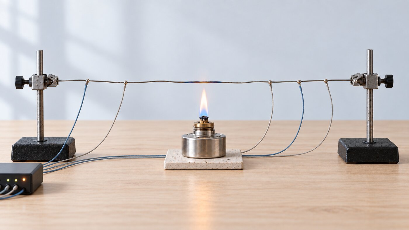
This can be modeled with the heat equation: the temperature field $T$ evolves as $$\partial_t T = \alpha \partial_{xx} T - \beta (T - T_0) + s,$$ where $\alpha$ is the heat diffusivity, $s$ a source term depending on position, and the second term describes relaxation to ambient temperature $T_0$ ³. At steady state, expressing the temperature relative to $T_0$ as $u = T - T_0$ and choosing units where $\beta=1$: $$u - l^2 \partial_{xx} u = s,$$ where $l = \sqrt{\alpha/\beta}$ is a length scale. If we solve this equation for a single point source $s(x) = \delta(x)$, the temperature takes the form $$u(x) = \frac{1}{2l} e^{-\frac{|x|}{l}},$$ which is also the Green function for this problem.

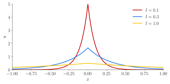
The temperature is a lot smoother than the source term since diffusion tends to smooth out any field.

When we know the source term, we can now predict the temperature profile, as it is given by the convolution between the source term and the Green function. But what if we do not know the source term?

The inverse problem

Suppose that instead of a known source term, we have measurements $\mathcal{D} = \{ \bar{u}_k \}_{k=1}^{N_D}$ of the rod temperature at given positions $\{ \bar{x}_k \}_{k=1}^{N_D}$. The measurements have errors, which we model as independent, normally distributed with a known standard deviation $\sigma$. Can we infer the temperature profile?

Two observations: this is an inverse problem, and there are uncertainties in the measurements, so we may treat the problem with a Bayesian approach. This is the approach taken by BODIL: represent the field on a grid, then define a likelihood and a prior, which together define the posterior distribution of the field.

Here the solution field, represented on a uniform grid, is the temperature over a rod of unit length, $u_i = u(x_i) = u(i \Delta x)$, where $\Delta x$ is the grid spacing. The likelihood is straightforward: we assume that the measurements are normally distributed around the solution field, giving $$P(\mathcal{D} \mid u) = \prod\limits_{k=1}^{N_D} \frac{1}{\sqrt{2\pi\sigma^2}} e^{-\frac{(\bar{u}_k - h_k(u))^2}{2\sigma^2}},$$ where $h_k$ is the interpolation of $u$ at the measurement location $\bar{x}_k$.

The prior contains the physics, encoded as a discretization of the PDE, here a central finite-difference scheme. Since we know nothing about the source, we encode it as white noise, with amplitude $\sigma_s$. This gives the following prior⁴: $$P(u) \propto \prod\limits_{i=1}^N \exp \left[ -\frac{\Delta x}{2 \sigma_s^2} \left( u_i - l^2 \frac{u_{i-1} - 2 u_i + u_{i+1}}{\Delta x^2}\right)^2 \right]$$ The following plot shows samples from this prior:

Despite the white noise assumption on the source, the temperature profiles are smooth! Putting everything together, we obtain the posterior:

We now have a reconstruction of the whole temperature profile, given sparse measurements and a physical prior, with quantified uncertainties. Note that we have used a finite number of grid points $N$, but changing $N$ barely changes the predictions. What happens, mathematically, in the continuum limit?

From prior to GP kernel

The continuum limit $\Delta x = 1 / N \rightarrow 0$ can help us understand BODIL as a GP. First, let's rewrite the log prior as $$\log P(u) = -\frac{\Delta x}{2\sigma_s^2} u^T R^T R u - \log Z,$$ where $R$ is the discrete residual operator, corresponding to $(1 - l^2 \Delta)$ in the continuum limit (we ignore boundary effects). The prior is thus a Gaussian with covariance $$\Sigma = \frac{\sigma_s^2}{\Delta x} \left(R^T R\right)^{-1}.$$ In the continuum limit, the question is whether $\Sigma_{ij}$ converges to a grid-independent kernel $k(x_i, x_j)$. We have seen earlier that solving $R u = s$ for $u$ in the continuum limit is a convolution of $s$ with the Green function $G(x) = e^{-|x|/l}/2l$. Therefore, $$\left(R^{-1} s\right)_i \approx \sum\limits_{j=1}^N G(x_i - x_j) s_j \Delta x,$$ for any $s$, giving $\left(R^{-1}\right)_{ij} \approx G(x_i - x_j) \Delta x$, and thus the covariance matrix reads $$\begin{aligned} \Sigma_{ij} &= \frac{\sigma_s^2}{\Delta x} \sum\limits_{k=1}^N \left(R^{-1}\right)_{ik} \left(R^{-T}\right)_{kj}, \\ &\approx \sigma_s^2 \sum\limits_{k=1}^N G(x_i - x_k) G(x_j - x_k) \Delta x, \\ &\rightarrow \sigma_s^2 \int G(x_i - y) G(x_j - y) dy, \end{aligned}$$ defining a kernel that does not depend on the grid size as $N \rightarrow \infty$. The kernel only depends on the distance $r = |x_j - x_i|$: $$k(r) = \sigma_s^2 \int G(r - y) G(y) dy = \frac{\sigma_s^2}{4l} \left(1 + \frac r l\right) e^{-\frac r l}.$$ What this means is that two nearby points are correlated, as they feel the same heat sources in their neighbourhood. This correlation vanishes once the points are further apart than $l$.

This is the Matérn kernel with $\nu = 3/2$ (in the usual parametrization, $\sigma^2 (1 + \sqrt{3} r / \rho) e^{-\sqrt{3} r / \rho}$, this corresponds to $\rho = \sqrt{3} l$ and $\sigma^2 = \sigma_s^2 / 4l$).

From posterior to GP regression

The posterior contains both the prior and the likelihood. The latter was defined with the interpolation operator $h_k$ for each of the $N_D$ data points, which we can write as a single $N_D \times N$ interpolation matrix $H$ so that $(Hu)_k = h_k(u)$. With these new notations the log-likelihood is expressed as $$\log P(\mathcal{D}|u) = -\frac{1}{2\sigma^2} \left(\bar{u} - H u\right)^T \left(\bar{u} - H u\right) - \frac{N_D}{2} \log{2\pi\sigma^2},$$ giving the log-posterior (up to an additive constant independent of $u$): $$\log P(u|\mathcal{D}) = - \frac 1 2 u^T \Sigma^{-1} u - \frac{1}{2\sigma^2} \left(\bar{u} - H u\right)^T \left(\bar{u} - H u\right) + \text{const},$$ which is a Gaussian with precision $Q_p = \Sigma^{-1} + H^TH / \sigma^2$ and mean $m = Q_p^{-1} H^T \bar u / \sigma^2$. Multiplying the latter by $\Sigma Q_p$ and rearranging gives $$\begin{equation} m = \Sigma H^T (\bar u - H m) / \sigma^2. \label{eq:mean} \end{equation}$$ Not very interpretable. Let's write it in terms of the (discrete) kernel.

We first define $a = (\bar u - H m) / \sigma^2$ and substitute it into $\eqref{eq:mean}$, to get $m = \Sigma H^T a$. Substituting this into the definition of $a$ gives $a = (\bar u - H \Sigma H^T a) / \sigma^2$, and thus $a= (H \Sigma H^T + \sigma^2 \mathbb{1})^{-1} \bar u$. Substituting this back into the mean, we have that $$\begin{equation} m = \Sigma H^T \left(H \Sigma H^T + \sigma^2 \mathbb{1} \right)^{-1} \bar u. \label{eq:gp:mean} \end{equation}$$ We can use a similar trick to get the covariance $\Sigma_p = Q_p^{-1}$ of the posterior: $$\begin{equation} \Sigma_p = \Sigma - \Sigma H^T \left(H \Sigma H^T + \sigma^2 \mathbb{1}\right)^{-1} H\Sigma. \label{eq:gp:cov} \end{equation}$$

In the continuum limit, $K(\bar{X}, \bar{X}) = H\Sigma H^T$ is the kernel evaluated between pairs of measurement points, and $\Sigma H^T$ is the kernel evaluated between grid points and measurement locations, $K(x, \bar{X})$. Here $\bar X$ denotes the positions of all measurements, and $K$ the matrix of kernel values between every pair of positions. Therefore, equation $\eqref{eq:gp:mean}$ corresponds to the GP regression formula $$\mathbb{E}\left[ u(x) \right] = K(x, \bar{X}) \left(K(\bar{X}, \bar{X}) + \sigma^2 \mathbb{1} \right)^{-1} \bar u,$$ and equation $\eqref{eq:gp:cov}$ corresponds to $$\mathrm{cov}\left[u(x), u(x')\right] = k(x, x') - K(x, \bar{X}) \left( K(\bar X, \bar X) + \sigma^2\mathbb{1} \right)^{-1} K(\bar{X}, x').$$ These are equations (2.23) and (2.24) in Rasmussen and Williams (2006).

In the GP form, evaluating the posterior at a new point requires first factorizing the dense $N_D \times N_D$ matrix, at a cost of $\mathcal O (N_D^3)$ operations. In the discrete case, we need to solve a linear system of size $N$ that is banded, since $R$ and $H$ only couple neighbouring grid points: its cost is linear in $N$ and independent of $N_D$, which may be a lot cheaper in some cases.

Summary

As a Bachelor student, I understood mathematical concepts best when they came with a physical picture: Fourier transforms through waves, differential equations through mechanics, stochastic processes through Brownian motion. GPs turn out to be no exception, and writing this post gave me the picture I was missing.

When the PDE is linear, solving the inverse problem with BODIL tends to GP regression as the grid is refined, and the kernel is the Green function of the PDE convolved with itself. Choosing a kernel is choosing a physics, whether one knows it or not.

When the PDE is non-linear, the posterior is not Gaussian anymore, and we have something more general than GPs. I might take a closer look at non-linear cases in a future post.

Footnotes